Constraints

Equations of motion for the \(k\)-th particle:

\[m_k\frac{d^2\mathbf{r}_k}{dt^2}=-\frac{\partial}{\partial \mathbf{r}_k}V\left(\{\mathbf{r}\}\right)=-\nabla_kV\left(\{\mathbf{r}\}\right)\]

Same equations with constraints:

\[m_k\frac{d^2\mathbf{r}_k}{dt^2}=-\frac{\partial}{\partial \mathbf{r}_k}\left(V\left(\{\mathbf{r}\}\right)+\sum_{c=1}^C\lambda_c\sigma_c\left(\{\mathbf{r}\}\right)\right)=\mathbf{f}_k+\delta\mathbf{f}_k\]

Where

\[\sigma_c\left(\{\mathbf{r}\}\right)=\mathbf{r}_{ml}^2-d_c^2=\mathbf{r}_{ml}^2-d_{ml}^2\]

Here, \(d_c=d_{ml}\) is the target distance between \(m\)-th and \(l\)-th particles (constrain \(c\) connects particles \(m\) and \(l\)).

The ‘’constrain’’ force \(\delta\mathbf{f}_k\) is then:

\[\delta\mathbf{f}_k=\frac{\partial}{\partial\mathbf{r}_k}\sum_{c=1}^{C}\lambda_c\sigma_c\left(\{\mathbf{r}\}\right)=\sum_{c=1}^{C}\lambda_c\frac{\partial}{\partial\mathbf{r}_k}\sigma_c\left(\{\mathbf{r}\}\right)=\sum_{c=1}^{C}\lambda_c2\delta_{km}\delta_{kl}\mathbf{r}_{ml}\]

Numerical integration

Since

\[m_k\frac{d^2\mathbf{r}_k}{dt^2}=\mathbf{f}_k+\delta\mathbf{f}_k\]

(add numerical scheme here to show how lambda and mu are related)

The numerical integration can be done in two steps: (1) integration as if there are no constraints and (2) adding the displacement due to ‘’constrain force’’ \(\delta\mathbf{f}_k\), so that the constraints are satisfied:

\[\mathbf{r}_k^{n+1}=\mathbf{r}_k^* + \delta\mathbf{r}_k\]

Where \(\mathbf{r}_k^*\) is the displaced coordinates as if there are no constraints and:

\[\delta\mathbf{r}_k=\sum_{c=1}^C\frac{\mu_c}{m_k}\left(\delta_{km}-\delta_{kl}\right)\mathbf{r}_{ml}\]

Here, \(\mu_c=2\lambda_c\tau^2\) is the normalized Lagrange multiplier.

Note that since \(\delta\mathbf{\upsilon}=\frac{\delta\mathbf{r}}{\tau}\), the scaled Lagrange multiplier for the velocities is \(\mu_c^\upsilon=\frac{\mu_c}{\tau}\).

Solving for \(\mu_c\)

For each constrain c, after the numerical integration, the distance between constrained atoms should be equal to the target distance of that constraint, \(d_c\). Hence, for each constraint we have \(|\mathbf{r}_{ij}^{n+1}|=d_{ij}\) or \({\mathbf{r}_{ij}^{n+1}}^2=d_{ij}^2\), where \(\mathbf{r}^{n+1}_{ij}=\mathbf{r}^{n+1}_{i}-\mathbf{r}^{n+1}_{j}\).

These conditions should be satisfied by finding appropriate values for \(\mu_c\) (or equally \(\lambda_c\)). The general form for these quadratic equations is:

\[\begin{split}\begin{split} \left(\mathbf{r}_{ij}^*+\delta\mathbf{r}_{ij}\right)^2-d_{ij}^2=0 \\ \left(\mathbf{r}_{ij}^*+\left(\delta\mathbf{r}_{i}-\delta\mathbf{r}_{j}\right)\right)^2-d_{ij}^2=0 \\ \left(\mathbf{r}_{ij}^*+\left(\sum_{c=1}^C\frac{\mu_c}{m_i}\left(\delta_{im}-\delta_{il}\right)\mathbf{r}_{ml} - \sum_{c=1}^C\frac{\mu_c}{m_j}\left(\delta_{jm}-\delta_{jl}\right)\mathbf{r}_{ml}\right)\right)^2-d_{ij}^2=0 \end{split}\end{split}\]

Finally:

(1)\[\left(\mathbf{r}_{ij}^*+\sum_{c=1}^C\mu_c\left(\frac{\delta_{im}-\delta_{il}}{m_i} - \frac{\delta_{jm}-\delta_{jl}}{m_j}\right)\mathbf{r}_{ml}\right)^2-d_{ij}^2=0\]

Note that the sum over all constraints \(c=\{m,l\}\) should include the pair \(\{i,j\}\), in which case only two of the kronecker’s deltas will survive. For a coupled constraint, when either \(i\) or \(j\) is equal to one index in the \(\{m,l\}\) pair, only one delta will not be zero. Since \(i\ne j\) and \(m\ne l\), there is never going to be the case when more than two deltas are not zero.

Notations

Before applying the above formula to specific cases, let us simplify the notations. First, let us us the \(r_i^0\) for the coordinates of the atom before the integration and \(r_i\) as the coordinates for the same particle after the integration and constraining is done. Second, let us assume that the constrain connecting atoms \(m\) and \(l\) has an index \(c\), and we will use the constraint index \(c\) and indices of the connected particles \(m\) and \(l\) interchangeably (we already did this for \(d_c=d_{ml}\) above). We will be assigning these indexes for each case before deriving the formulas. This should allow us to have less noise in the formulas and the generalization for the \(n\)-th step and for arbitrary indices of particles should be straightforward.

One constraint

The simplest case by far is when we have a single constraint, which is not coupled to any other. An example should be the constrained C-H bond in the protein backbone in the case when only bonds with hydrogens are constrained (with the only exception of glycine, where there is another hydrogen instead of a side-chain). Indeed, this case is very simple: we have the direction of the bond in which atoms should be moved. And the sum of the displacements for two moved atoms should be so that the final distance is equal to the target. The displacements are reversely proportional to masses of atoms. Let us derive this formally, using the Equation 1 above.

../../_images/CH1.png

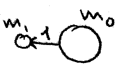
Fig. 6 A schematic representation of a constrained bond. Index on top of the bond represents the constraint index \(c\). Arrow indicates the direction of the vector \(\mathbf{r}_1\). Masses subscripts correspond to aton indices.

We have one constraint \(c=1=\{0,1\}\) that connects two atoms \(i=0\) and \(j=1\) with masses \(m_0\) and \(m_1\). We will also denote all the connecting vectors with constrain index, i.e. \(\mathbf{r}_1=\mathbf{r}_{01}=\mathbf{r}_0-\mathbf{r}_1\), etc. so there is less noise in formulas. Note that we could remove the index altogether since there is only one constrained bond, but we will keep the index here for consistency with the rest of the cases. The sole equation derived from Equation 1 is:

\[\left(\mathbf{r}_{1}^*+\mu_1\left(\frac{1}{m_0}+\frac{1}{m_1}\right)\mathbf{r}_1^0\right)^2-d_1^2=0\]

With reduced mass \(M_1=\frac{m_0m_1}{m_0+m_1}\):

\[\left(\mathbf{r}_{1}^*+\frac{\mu_1}{M_1}\mathbf{r}_1^0\right)^2-d_1^2=0\]

Expanding:

(2)\[\mu_1^2\frac{{\mathbf{r}_1^0}^2}{M_1^2}+2\mu_1\frac{\left(\mathbf{r}_1^*\cdot\mathbf{r}_1^0\right)}{M_1}+\left({\mathbf{r}_1^*}^2-d_1^2\right)=0\]

This is a single quadratic equation for \(\mu_1\), with the following solution:

\[\begin{split}\begin{split} D_2=\frac{1}{M_1^2}\left(\left(\mathbf{r}_1^*\cdot\mathbf{r}_1^0\right)^2-{\mathbf{r}_1^0}^2\left({\mathbf{r}_1^*}^2-d_1^2\right)\right) \\ {\mu_1}^{1,2}=\frac{\pm\sqrt{D_2}-\frac{\left(\mathbf{r}_1^*\cdot\mathbf{r}_1^0\right)}{M_1}}{\frac{{\mathbf{r}_1^0}^2}{M_1^2}} \end{split}\end{split}\]

Plugging the \(D_2\) into the solution gives:

\[{\mu_1}^{1,2}=M_1\frac{\pm\sqrt{\left(\left(\mathbf{r}_1^*\cdot\mathbf{r}_1^0\right)^2-{\mathbf{r}_1^0}^2\left({\mathbf{r}_1^*}^2-d_1^2\right)\right)}-\left(\mathbf{r}_1^*\cdot\mathbf{r}_1^0\right)}{{\mathbf{r}_1^0}^2}\]

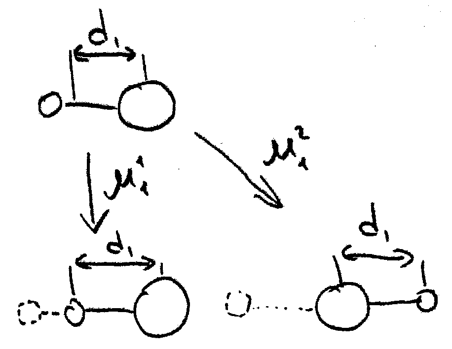
As expected for quadratic equation, we have two solutions. However only one is valid for our problem: the one that gives smaller absolute value of \(\mu\). This is because we assume that the bond length after the numerical integration without constraints is close to the target length, i.e. the displacements of the atoms is small. Indeed, we can move the atoms so they satisfy the constraint two ways, one of which employs flipping the bond.

../../_images/CH1_mu12.png

Fig. 7 Two roots give two different directions of the bond after constraining. Given that the timestep is small, the displacement should be small as well. Hence the correct solution for \(\mu_1\) is the smallest by absolute value.

The solution we are interested in is the one with the plus sign before the square root. So the final solution for \(\mu_1\) is:

(3)\[\mu_1=M_1\frac{\sqrt{\left(\left(\mathbf{r}_1^*\cdot\mathbf{r}_1^0\right)^2-{\mathbf{r}_1^0}^2\left({\mathbf{r}_1^*}^2-d_1^2\right)\right)}-\left(\mathbf{r}_1^*\cdot\mathbf{r}_1^0\right)}{{\mathbf{r}_1^0}^2}\]

Though this equation is quite simple, we need to prepare ourselves to the following cases. So let us introduce the notations for all the coefficients in the Equation 2, re-writing it as:

\[k_1^{11}\mu_1^2+k_1^1\mu_1+k_1^0=0\]

Here, the indices for parameters \(k_x^y\) are chosen the following way. The bottom index is the number of equation (we have one so far). The top indexes indicate what combination of variables \(mu\) this coefficient is multiplied by: \(k_1^{11}\) is for \(\mu_1\mu_1=\mu^2\), \(k_1^1\) is for \(\mu_1\) and \(0\) is for free coefficient. Later we will encounter other variables (\(\mu_2\), \(\mu_3\), etc.), for which we will have \(k_1^{22}\), \(k_1^{33}\) as well as some mixed products, e.g. \(\mu_1\mu_2\) with \(k_1^{12}\), etc. As follows from Equation 2, in the case of one uncoupled constraint, there are three coefficient:

\[k_1^{11}=\frac{{\mathbf{r}_1^0}^2}{M_1^2}\mathrm{,~~} k_1^1=\frac{2\left(\mathbf{r}_1^*\cdot\mathbf{r}_1^0\right)}{M_1}\mathrm{,~~} k_1^0={\mathbf{r}_1^*}^2-d_1^2\]

In these notations, the solution for \(\mu_1\) is:

(4)\[\mu_1=\frac{\sqrt{{k_1^1}^2-4k_1^{11}k_1^0}-k_1^1}{2k_1^{11}}\]

Note, that using Equation 4 is slightly less computationally efficient when compared to Equation 3.

Two coupled constraints

../../_images/CH2.png

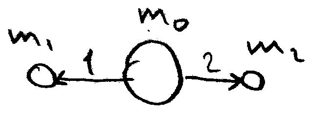
Fig. 8 A schematic representation of two coupled constrained bonds.

Two coupled constraints will give us a much more complicated case of two coupled quadratic equations. Assuming that the central atom has index \(0\), with atoms \(1\) and \(2\) connected to it with two constrained bonds \(c=1=\{0,1\}\) and \(c=2=\{0.2\}\), and using the reduced masses \(M_1=\frac{m_0m_1}{m_0+m_1}\) and \(M_2=\frac{m_0m_2}{m_0+m_2}\), from Equation 1 we get:

\[\begin{split}\begin{cases} \left(\mathbf{r}_{1}^*+\frac{\mu_1}{M_1}\mathbf{r}_1^0+\frac{\mu_2}{m_0}\mathbf{r}_2^0\right)^2-d_1^2=0 \\ \left(\mathbf{r}_{2}^*+\frac{\mu_1}{m_0}\mathbf{r}_1^0+\frac{\mu_2}{M_2}\mathbf{r}_2^0\right)^2-d_2^2=0 \end{cases}\end{split}\]
(5)\[\begin{split}\begin{cases} k_1^{11}\mu_1^2+k_1^{22}\mu_2^2+k_1^{12}\mu_1\mu_2+k_1^1\mu_1+k_1^2\mu_2+k_1^0=0 \\ k_2^{11}\mu_1^2+k_2^{22}\mu_2^2+k_2^{12}\mu_1\mu_2+k_2^1\mu_1+k_2^2\mu_2+k_2^0=0 \end{cases}\end{split}\]

Where

(6)\[\begin{split}\begin{split} k_1^{11}=\frac{{\mathbf{r}_1^0}^2}{M_1^2}\mathrm{,~~} k_1^{22}=\frac{{\mathbf{r}_2^0}^2}{m_0^2}\mathrm{,~~} k_1^{12}=\frac{2\left(\mathbf{r}_1^0\cdot\mathbf{r}_2^0\right)}{M_1m_0}\mathrm{,} \\ k_1^1=\frac{2\left(\mathbf{r}_1^*\cdot\mathbf{r}_1^0\right)}{M_1}\mathrm{,~~} k_1^2=\frac{2\left(\mathbf{r}_1^*\cdot\mathbf{r}_2^0\right)}{m_0}\mathrm{,~~} k_1^0={\mathbf{r}_1^*}^2-d_1^2\mathrm{,~~} \\ \\ k_2^{11}=\frac{{\mathbf{r}_1^0}^2}{m_0^2}\mathrm{,~~} k_2^{22}=\frac{{\mathbf{r}_2^0}^2}{M_2^2}\mathrm{,~~} k_2^{12}=\frac{2\left(\mathbf{r}_1^0\cdot\mathbf{r}_2^0\right)}{M_2m_0}\mathrm{,} \\ k_2^1=\frac{2\left(\mathbf{r}_2^*\cdot\mathbf{r}_1^0\right)}{m_0}\mathrm{,~~} k_2^2=\frac{2\left(\mathbf{r}_2^*\cdot\mathbf{r}_2^0\right)}{M_2}\mathrm{,~~} k_2^0={\mathbf{r}_2^*}^2-d_2^2\mathrm{.} \end{split}\end{split}\]

Equation 5 are two coupled quadratic equations of a general form. Unfortunately, there is no simple analytical solution to it. Hence the numerical method should be used. Before describing the methods used currently in most MD software packages, let us try to introduce a method for the specific cases we are considering here.

If we introduce two dimensional vector-function \(F(\mu_1, \mu_2)\) in Equation 5 it becomes:

\[\mathbf{F}(\mu_1, \mu_2) = \mathbf{0}\]

This is a system of non-linear equations, which are notoriously hard to solve if we (1) need to find all the solutions and (2) don’t have good initial guess for these solutions. However, this is not the case here. Firstly, we assume that atoms did satisfy the constraints on the previous step (i.e. we are looking for \(mu\)’s with smallest absolute value). Secondly, we only need to find this solution (see how we dropped one of the roots when solving for uncoupled constraint). Hence we can apply the Newtons method (also known as Newton-Raphson method). The general form of in in multi-dimensional case is:

(7)\[\mathbf{\mu}^{n+1}=\mathbf{\mu}^n-J_\mathbf{F}\left(\mathbf{\mu}^n\right)^{-1}\mathbf{F}\left(\mathbf{\mu}^n\right)\]

Here, \(\mathbf{\mu}^n=(\mu_1^n,\mu_2^n)^T\) is a vector with the solutions on \(n\)-th iteration, \(J_\mathbf{F}\left(\mathbf{\mu}\right)=J_\mathbf{F}\left(\mu_1, \mu_2\right)\) is the Jakobian matrix for the system. Using Equation 5, we can compute \(J_\mathbf{F}\left(\mu_1, \mu_2\right)\):

\[\begin{split}J_\mathbf{F}= \begin{pmatrix} 2k_1^{11}\mu_1+k_1^{12}\mu_2+k_1^1 & k_1^{12}\mu_1+2k_1^{22}\mu_2+k_1^2 \\ 2k_2^{11}\mu_1+k_2^{12}\mu_2+k_2^1 & k_1^{12}\mu_2+2k_2^{22}\mu_2+k_2^2 \end{pmatrix}\end{split}\]

With everything in the Equation 7 derived, we need good initial approximation for \(\mu_1\) and \(mu_2\). One can use zeroes, assuming that atoms did not moved much during the integration time step atoms did not moved far away from their previous positions (which did satisfy the constraints). We can get slightly better initial approximation by assuming that the constraints are not coupled, i.e. by using Equation 3 or Equation 4 for two constraints we have in our case:

(8)\[\begin{split}\begin{split} \mu_1^0=\frac{\sqrt{{k_1^1}^2-4k_1^{11}k_1^0}-k_1^1}{2k_1^{11}} \\ \mu_2^0=\frac{\sqrt{{k_2^2}^2-4k_2^{22}k_2^0}-k_2^2}{2k_2^{22}} \end{split}\end{split}\]

The numerical procedure to evaluate \(\mu_1\) and \(\mu_2\) is then contains following steps. (1) Compute coefficients in Equation 6. (2) Use Equation 8 to get initial approximations \(\mu_1^0\) and \(\mu_2^0\) for \(\mu_1\) and \(\mu_2\). (3) Compute \(\mathbf{F}(\mu_1, \mu_2)\) using Equation 5 and \(J_\mathbf{F}\left(\mu_1, \mu_2\right)\), invert the matrix \(J_\mathbf{F}\) (one can derive formulas to compute the inverse Jakobian directly, without computing the Jakobian itself). (4) Apply the Equation 7 to get the next iteration values for \(\mu_1\) and \(\mu_2\). (5) Repeat steps (3) and (4) until convergence.

Three constraints coupled through the central atom

../../_images/CH3.png

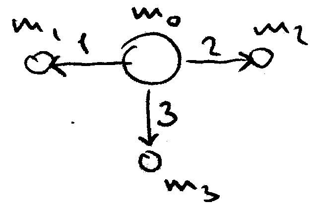
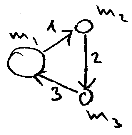
Fig. 9 A schematic representation of three atoms constrained to one central atom.

\[\begin{split}\begin{cases} \left(\mathbf{r}_{1}^*+\frac{\mu_1}{M_1}\mathbf{r}_1^0+\frac{\mu_2}{m_0}\mathbf{r}_2^0+\frac{\mu_3}{m_0}\mathbf{r}_3^0\right)^2-d_1^2=0 \\ \left(\mathbf{r}_{2}^*+\frac{\mu_1}{m_0}\mathbf{r}_1^0+\frac{\mu_2}{M_2}\mathbf{r}_2^0+\frac{\mu_3}{m_0}\mathbf{r}_3^0\right)^2-d_2^2=0 \\ \left(\mathbf{r}_{3}^*+\frac{\mu_1}{m_0}\mathbf{r}_1^0+\frac{\mu_2}{m_0}\mathbf{r}_2^0+\frac{\mu_3}{M_3}\mathbf{r}_3^0\right)^2-d_3^2=0 \\ \end{cases}\end{split}\]
(9)\[\begin{split}\begin{cases} k_1^{11}\mu_1^2+k_1^{22}\mu_2^2+k_1^{33}\mu_3^2+k_1^{12}\mu_1\mu_2+k_1^{13}\mu_1\mu_3+k_1^{23}\mu_2\mu_3+k_1^1\mu_1+k_1^2\mu_2+k_1^3\mu_3+k_1^0=0 \\ k_2^{11}\mu_1^2+k_2^{22}\mu_2^2+k_2^{33}\mu_3^2+k_2^{12}\mu_1\mu_2+k_2^{13}\mu_1\mu_3+k_2^{23}\mu_2\mu_3+k_2^1\mu_1+k_2^2\mu_2+k_2^3\mu_3+k_2^0=0 \\ k_3^{11}\mu_1^2+k_3^{22}\mu_2^2+k_3^{33}\mu_3^2+k_3^{12}\mu_1\mu_2+k_3^{13}\mu_1\mu_3+k_3^{23}\mu_2\mu_3+k_3^1\mu_1+k_3^2\mu_2+k_3^3\mu_3+k_3^0=0 \end{cases}\end{split}\]

Where

(10)\[\begin{split}\begin{split} k_1^{11}=\frac{{\mathbf{r}_1^0}^2}{M_1^2}\mathrm{,~~} k_1^{22}=\frac{{\mathbf{r}_2^0}^2}{m_0^2}\mathrm{,~~} k_1^{33}=\frac{{\mathbf{r}_3^0}^2}{m_0^2}\mathrm{,} \\ k_1^{12}=\frac{2\left(\mathbf{r}_1^0\cdot\mathbf{r}_2^0\right)}{M_1m_0}\mathrm{,~~} k_1^{13}=\frac{2\left(\mathbf{r}_1^0\cdot\mathbf{r}_3^0\right)}{M_1m_0}\mathrm{,~~} k_1^{23}=\frac{2\left(\mathbf{r}_2^0\cdot\mathbf{r}_3^0\right)}{m_0^2}\mathrm{,} \\ k_1^1=\frac{2\left(\mathbf{r}_1^*\cdot\mathbf{r}_1^0\right)}{M_1}\mathrm{,~~} k_1^2=\frac{2\left(\mathbf{r}_1^*\cdot\mathbf{r}_2^0\right)}{m_0}\mathrm{,~~} k_1^3=\frac{2\left(\mathbf{r}_1^*\cdot\mathbf{r}_3^0\right)}{m_0}\mathrm{,~~} k_1^0={\mathbf{r}_1^*}^2-d_1^2\mathrm{,~~} \\ \\ k_2^{11}=\frac{{\mathbf{r}_1^0}^2}{m_0^2}\mathrm{,~~} k_2^{22}=\frac{{\mathbf{r}_2^0}^2}{M_2^2}\mathrm{,~~} k_2^{33}=\frac{{\mathbf{r}_3^0}^2}{m_0^2}\mathrm{,} \\ k_2^{12}=\frac{2\left(\mathbf{r}_1^0\cdot\mathbf{r}_2^0\right)}{M_2m_0}\mathrm{,~~} k_2^{13}=\frac{2\left(\mathbf{r}_1^0\cdot\mathbf{r}_3^0\right)}{m_0^2}\mathrm{,~~} k_2^{23}=\frac{2\left(\mathbf{r}_2^0\cdot\mathbf{r}_3^0\right)}{M_2m_0}\mathrm{,} \\ k_2^1=\frac{2\left(\mathbf{r}_2^*\cdot\mathbf{r}_1^0\right)}{m_0}\mathrm{,~~} k_2^2=\frac{2\left(\mathbf{r}_2^*\cdot\mathbf{r}_2^0\right)}{M_2}\mathrm{,~~} k_2^3=\frac{2\left(\mathbf{r}_2^*\cdot\mathbf{r}_3^0\right)}{m_0}\mathrm{,~~} k_2^0={\mathbf{r}_2^*}^2-d_2^2\mathrm{,~~} \\ \\ k_3^{11}=\frac{{\mathbf{r}_1^0}^2}{m_0^2}\mathrm{,~~} k_3^{22}=\frac{{\mathbf{r}_2^0}^2}{m_0^2}\mathrm{,~~} k_3^{33}=\frac{{\mathbf{r}_3^0}^2}{M_3^2}\mathrm{,} \\ k_3^{12}=\frac{2\left(\mathbf{r}_1^0\cdot\mathbf{r}_2^0\right)}{m_0^2}\mathrm{,~~} k_3^{13}=\frac{2\left(\mathbf{r}_1^0\cdot\mathbf{r}_3^0\right)}{M_3m_0}\mathrm{,~~} k_3^{23}=\frac{2\left(\mathbf{r}_2^0\cdot\mathbf{r}_3^0\right)}{M_3m_0}\mathrm{,} \\ k_3^1=\frac{2\left(\mathbf{r}_3^*\cdot\mathbf{r}_1^0\right)}{m_0}\mathrm{,~~} k_3^2=\frac{2\left(\mathbf{r}_3^*\cdot\mathbf{r}_2^0\right)}{m_0}\mathrm{,~~} k_3^3=\frac{2\left(\mathbf{r}_3^*\cdot\mathbf{r}_3^0\right)}{M_3}\mathrm{,~~} k_3^0={\mathbf{r}_3^*}^2-d_3^2\mathrm{,~~} \\ \\ \end{split}\end{split}\]
\[\begin{split}\begin{split} &J_\mathbf{F}=\\ &\begin{pmatrix} 2k_1^{11}\mu_1+k_1^{12}\mu_2+k_1^{13}\mu_3+k_1^1 & k_1^{12}\mu_1+2k_1^{22}\mu_2+k_1^{23}\mu_3+k_1^2 & k_1^{13}\mu_1+k_1^{23}\mu_2+2k_1^{33}\mu_3+k_1^3 \\ 2k_2^{11}\mu_1+k_2^{12}\mu_2+k_2^{13}\mu_3+k_2^1 & k_2^{12}\mu_1+2k_2^{22}\mu_2+k_2^{23}\mu_3+k_2^2 & k_2^{13}\mu_1+k_2^{23}\mu_2+2k_2^{33}\mu_3+k_2^3 \\ 2k_3^{11}\mu_1+k_3^{12}\mu_2+k_3^{13}\mu_3+k_3^1 & k_3^{12}\mu_1+2k_3^{22}\mu_2+k_3^{23}\mu_3+k_3^2 & k_3^{13}\mu_1+k_3^{23}\mu_2+2k_3^{33}\mu_3+k_3^3 \\ \end{pmatrix} \end{split}\end{split}\]

Triangle of constraints

../../_images/H2O.png

Fig. 10 Three constraints can form a rigid triangle, e.g. in water molecule.

\[\begin{split}\begin{cases} \left(\mathbf{r}_{1}^*+\frac{\mu_1}{M_1}\mathbf{r}_1^0-\frac{\mu_2}{m_2}\mathbf{r}_2^0-\frac{\mu_3}{m_1}\mathbf{r}_3^0\right)^2-d_1^2=0 \\ \left(\mathbf{r}_{2}^*-\frac{\mu_2}{m_0}\mathbf{r}_1^0+\frac{\mu_2}{M_2}\mathbf{r}_2^0-\frac{\mu_3}{m_3}\mathbf{r}_3^0\right)^2-d_2^2=0 \\ \left(\mathbf{r}_{3}^*-\frac{\mu_1}{m_1}\mathbf{r}_1^0-\frac{\mu_3}{m_0}\mathbf{r}_2^0+\frac{\mu_3}{M_3}\mathbf{r}_3^0\right)^2-d_3^2=0 \\ \end{cases}\end{split}\]
(11)\[\begin{split}\begin{split} k_1^{11}=\frac{{\mathbf{r}_1^0}^2}{M_1^2}\mathrm{,~~} k_1^{22}=\frac{{\mathbf{r}_2^0}^2}{m_2^2}\mathrm{,~~} k_1^{33}=\frac{{\mathbf{r}_3^0}^2}{m_1^2}\mathrm{,} \\ k_1^{12}=-\frac{2\left(\mathbf{r}_1^0\cdot\mathbf{r}_2^0\right)}{M_1m_2}\mathrm{,~~} k_1^{13}=-\frac{2\left(\mathbf{r}_1^0\cdot\mathbf{r}_3^0\right)}{M_1m_1}\mathrm{,~~} k_1^{23}=\frac{2\left(\mathbf{r}_2^0\cdot\mathbf{r}_3^0\right)}{m_1m_2}\mathrm{,} \\ k_1^1=\frac{2\left(\mathbf{r}_1^*\cdot\mathbf{r}_1^0\right)}{M_1}\mathrm{,~~} k_1^2=-\frac{2\left(\mathbf{r}_1^*\cdot\mathbf{r}_2^0\right)}{m_2}\mathrm{,~~} k_1^3=-\frac{2\left(\mathbf{r}_1^*\cdot\mathbf{r}_3^0\right)}{m_1}\mathrm{,~~} k_1^0={\mathbf{r}_1^*}^2-d_1^2\mathrm{,~~} \\ \\ k_2^{11}=\frac{{\mathbf{r}_1^0}^2}{m_2^2}\mathrm{,~~} k_2^{22}=\frac{{\mathbf{r}_2^0}^2}{M_2^2}\mathrm{,~~} k_2^{33}=\frac{{\mathbf{r}_3^0}^2}{m_3^2}\mathrm{,} \\ k_2^{12}=-\frac{2\left(\mathbf{r}_1^0\cdot\mathbf{r}_2^0\right)}{M_2m_2}\mathrm{,~~} k_2^{13}=\frac{2\left(\mathbf{r}_1^0\cdot\mathbf{r}_3^0\right)}{m_2m_3}\mathrm{,~~} k_2^{23}=-\frac{2\left(\mathbf{r}_2^0\cdot\mathbf{r}_3^0\right)}{M_2m_3}\mathrm{,} \\ k_2^1=-\frac{2\left(\mathbf{r}_2^*\cdot\mathbf{r}_1^0\right)}{m_2}\mathrm{,~~} k_2^2=\frac{2\left(\mathbf{r}_2^*\cdot\mathbf{r}_2^0\right)}{M_2}\mathrm{,~~} k_2^3=-\frac{2\left(\mathbf{r}_2^*\cdot\mathbf{r}_3^0\right)}{m_3}\mathrm{,~~} k_2^0={\mathbf{r}_2^*}^2-d_2^2\mathrm{,~~} \\ \\ k_3^{11}=\frac{{\mathbf{r}_1^0}^2}{m_1^2}\mathrm{,~~} k_3^{22}=-\frac{{\mathbf{r}_2^0}^2}{m_3^2}\mathrm{,~~} k_3^{33}=-\frac{{\mathbf{r}_3^0}^2}{M_3^2}\mathrm{,} \\ k_3^{12}=\frac{2\left(\mathbf{r}_1^0\cdot\mathbf{r}_2^0\right)}{m_1m_3}\mathrm{,~~} k_3^{13}=-\frac{2\left(\mathbf{r}_1^0\cdot\mathbf{r}_3^0\right)}{M_3m_1}\mathrm{,~~} k_3^{23}=-\frac{2\left(\mathbf{r}_2^0\cdot\mathbf{r}_3^0\right)}{M_3m_3}\mathrm{,} \\ k_3^1=-\frac{2\left(\mathbf{r}_3^*\cdot\mathbf{r}_1^0\right)}{m_1}\mathrm{,~~} k_3^2=-\frac{2\left(\mathbf{r}_3^*\cdot\mathbf{r}_2^0\right)}{m_3}\mathrm{,~~} k_3^3=\frac{2\left(\mathbf{r}_3^*\cdot\mathbf{r}_3^0\right)}{M_3}\mathrm{,~~} k_3^0={\mathbf{r}_3^*}^2-d_3^2\mathrm{,~~} \\ \\ \end{split}\end{split}\]

Note that \(\left(\mathbf{r}_1^0\cdot\mathbf{r}_2^0\right)=\left(\mathbf{r}_2^0\cdot\mathbf{r}_3^0\right)=\left(\mathbf{r}_3^0\cdot\mathbf{r}_1^0\right)=-2S_0\), where \(S_0\) is the area of the triangle.

SETTLE

The triangle of constraints case is very common for the biomolecular simulations since most of water models constrain both bonds between hydrogens and oxygen and H-O-H angle. And there is an analytical solution for this specific case, called SETTLE [Miyamoto and Kollman, 1992]. This algorithm is in fact used in most of the MD software. In brief, the idea of SETTLE is first to reduce the problem into two dimensions, and than compute the rotation angle of the constraints triangle using two-dimensional Euler angles.

More than three coupled constraints

We can keep expanding our formulas to the cases with more coupled constraints, and they will get more and more complex. However, there are only a few cases that is useful to solve this way: four constraints coupled to the central (e.g. methane molecule) atom and various rings that should be kept planar (e.g. benzene ring in phenylalanine or double ring in the tryptophane side-chain). These are not very common, the rings are usually kept planar with improper dihedral potentials, so we will not derive them here. Much more important is the case where all covalent bonds are constraints, where universal formalism is needed. The two most common algorithms for this case are SHAKE [J.P. Ryckaert and Berendsen, 1977] (and its “velocity version” RATTLE [Andersen, 1983]) and LINCS [Hess, 2008, Hess et al., 1997]. Note that the latter is the default option in GROMACS.

1

H.C. Andersen. RATTLE: A “velocity” version of the shake algorithm for molecular dynamics calculations. J. Comput. Phys., 52(1):24–34, 1983. doi:10.1016/0021-9991(83)90014-1.

2

B. Hess. P-LINCS: A parallel linear constraint solver for molecular simulation. J. Chem. Theory Comput., 4(1):116–122, 2008. doi:10.1021/ct700200b.

3

B. Hess, H. Bekker, H.J.C. Berendsen, and J.G.E.M. Fraaije. LINCS: A linear constraint solver for molecular simulations. J. Comput. Chem., 18(12):1463–1472, 1997. doi:10.1002/(SICI)1096-987X(199709)18:12<1463::AID-JCC4>3.0.CO;2-H.

4

J.P. Ryckaert, G. Ciccotti and H.J.C. Berendsen. Numerical integration of the cartesian equations of motion of a system with constraints: Molecular Dynamics of n-alkanes. J. Comp. Phys., 23(3):327–341, 1977. doi:10.1016/0021-9991(77)90098-5.

5

S. Miyamoto and P.A. Kollman. SETTLE: An analytical version of the SHAKE and RATTLE algorithm for rigid water models. J. Comput. Chem., 13(8):952–962, 1992. doi:10.1002/jcc.540130805.